Probability Distributions
- Dr. Bhupender Kumar Som
- Oct 17, 2022
- 4 min read

Updated: Dec 6, 2022

Before understanding the probability distribution, we shall understand the concept of a random variable also known as chance or stochastic variable is the variable that contains the outcome of a chance experiment is known as a random variable. For instance, in outcome of toss of three coins, the random variable can be defined as, “x": number of heads obtained”. This random variable ‘x’ can take values 0, 1, 2 or 3. In the example above the nature of the random variable is discrete in nature and hence the random variable is called a discrete random variable. In other example if the random variable is represented by the height of a student in the particular institute, then the random variable can take any value between shortest and tallest student and hence called as a continuous random variable.
The probability distribution associated with a random variable can be defined as per following example. Consider a simultaneous throw of three coins, this random experiment may result in any of the following eight outcomes. (HHH), (HHT), (HTT), (TTT), (TTH), (THH), (THT), (HTH). Now consider random variable ‘x’ as number of heads obtained. ‘x’ can take values 0, 1, 2, or 3 i.e., observer can get either no head, 1 head, 2 heads or 3 heads at-most. The probability distribution of these outcomes cab be given by

Since the variable under study is discrete in nature, hence the probability distribution under study is called discrete probability distribution. Likewise, the probability distribution w.r.t. continuous random variable can be studied and is known as continuous probability distribution. For example, the random variable ‘y’ represents the height of a student in a particular institution consisting of 200 students and varies from 4 feet 9 inches to 6 feet 3 inches. The probability distribution may be given by.

Further the Probability distributions can be studied as.
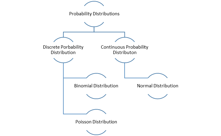
Binomial Porbability Distribution
Given by one of the eight mathematicians in Bernoulli family, James Bernoulli, born in Basel Switzerland on December 27, 1654 and died on August 16, 1705. Binomial Probability Distribution is based on the idea that every random experiment can be considered resulting in two possible outcomes i.e., happening of the particular event of interest and not-happening of that particular event of interest. It can also be called as success or failure. The experiment that results in two possible outcomes is known as Bernoulli’s experiment or Binomial Experiment. These outcomes are.
1. Mutually Exclusive
2. Collectively Exhaustive
3. Sum of their probabilities is 1.
Success in the experiment is called as Binomial random variable and its distribution is called Binomial Distribution.
Conditions Necessary for Binomial Distribution
Each trail has only two possible outcomes called success and failure
There are finite number of trials
All trials are identical i.e., the probability of success is same for each trail
The trails are independent to each other
Parameters of Binomial Distribution
There are two parameters of Binomial Distribution
Number of trails, i.e., ‘n’.
Probability of success in each trail i.e., p
Probability Distribution Function of “Binomial Distribution” can be given by

Where, 'n', represents the number of trails, 'x' represents the number of successes, 'p', represents the probability of success in each trail and 'q', is represented by q = 1 - p.

Video tutorial: Solving Binomial Probability Distribution problems using MS Excel
Poisson Probability Distribution


Video tutorial: Solving Poisson Probability Distribution problems using MS Excel
Normal Probability Distribution
Normal distribution is a continuous probability distribution given by Carl Fedrich Gauss, A German Mathematician. As the random variable under study is continuous in nature the distribution is continuous in nature. It is one of the most widely used probability distribution. A large number of datasets in the universe follow a bell shaped curved called as normal curve i.e. most of the observations collate around the mean value.
The normal distribution plays a key role in business decisions. The distribution is highly useful for making inferences for population where only sample information is available. The normal distribution can also be said as limiting case of Binomial and Poisson distribution under different conditions.
The Normal Curve
Assume a data set of income of the people in a population is given as follows
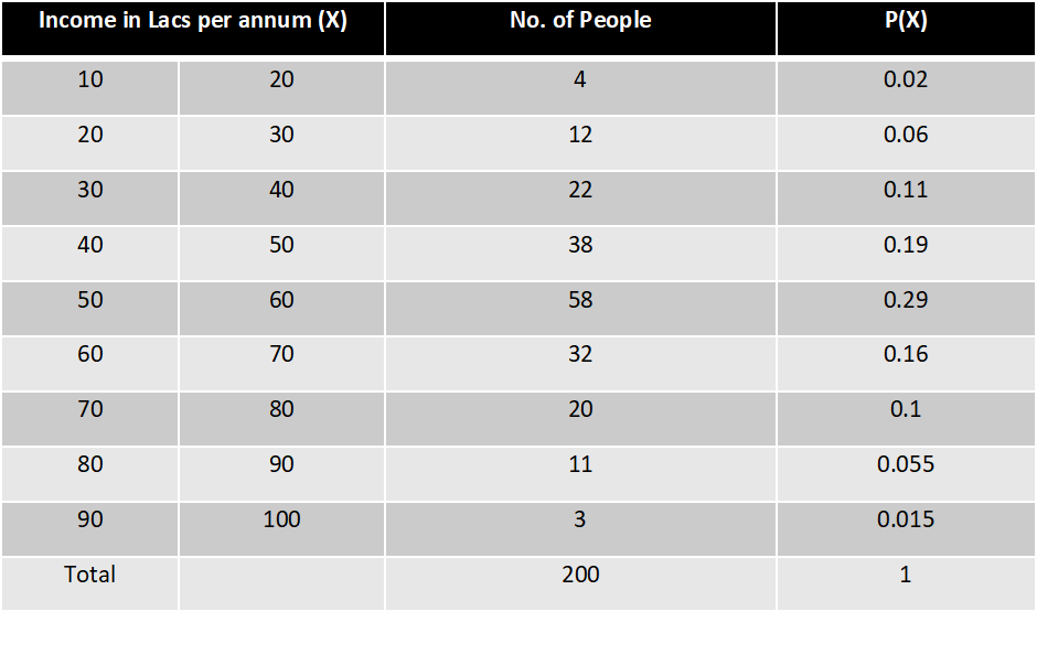
If we plot this data using a histogram, having income (X) on X-axis and Probability of X, P(X) on Y-axis we get following diagram
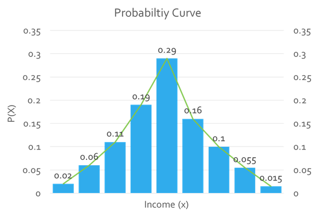
This figure shows that data is following a bell shaped curve or also called as a normal curve. The probability of random variable ‘x’ is taken on Y axis and the random variable representing income is taken on x-axis. Gauss has given the idea of standard normal curve for all continuous random variables. He mentioned that all continuous random variables can be converted into a standard normal variate z using following formula


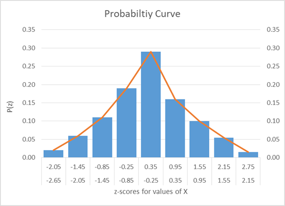
The mean and standard deviation for X and standard normal variate of X i.e., z is given by


The total probability under the curve remains equal to 1
The curve is symmetric about the Y- axis i.e., left side of the curve is mirror image of the right.
The curve has its peak at the mean value and tapers down to x-axis from both tails but never touches it.
The curve has a mean equal to ‘0’ and standard deviation equal to ‘1’.
The X – axis of the curve denotes the scores of standard normal variate z and the Y-axis of the curve denotes P (z).
The area under the curve is given by a table named as area under the normal curve. The snapshot of it is given below.

Video Tutorial: Solving Normal Distribution Problem using MS Excel


Comments